Introduction to Lambda Architecture

This post is a part of a series on Lambda Architecture consisting of:

• Introduction to Lambda Architecture
• Implementing Data Ingestion using Apache Kafka, Tweepy
• Implementing Batch Layer using Kafka, S3, Redshift
• Implementing Speed Layer using Spark Structured Streaming
• Implementing Serving Layer using Redshift

You can find a Youtube playlist explaining the code and results for each of the topics here and you can find the source code of the series here.

---

Contents

• What is lambda architecture
• Example of lambda architecture using Kafka, Spark Streaming, S3, Redshift

What is Lambda architecture

Definiton from wikipedia:

Lambda architecture is a data-processing architecture designed to handle massive quantities of data by taking advantage of both batch and stream processing methods. This approach to architecture attempts to balance latency, throughput, and fault-tolerance by using batch processing to provide comprehensive and accurate views of batch data, while simultaneously using real-time stream processing to provide views of online data. The two view outputs may be joined before presentation.

Lambda architecture consists of three main components:

1. batch layer

2. speed layer

3. serving layer

Batch layer

Batch layer provides the functionality of append-only set of raw data and computed batch views.

The batch layer looks at all of the historical data and serves as the single version of the truth by processing all available data when generating views.

It serves as correction of the speed layer because it can aggregate large volumes of historical data and provides full fault tolerance unlike streaming systems.

Speed layer

Speed layer processes data streams in real time to accomodate low latency requests for data.

It is responsible for filling the gap between the latest batch view and real time data.

By operating on smaller windows of data it can provide fast, real time views of real time data.

Serving layer

Serving layer merges together the outputs of batch and speed layers to provide the lowest latency and highest accuracy responses to users queries.

---

Example of lambda architecture using Kafka, Spark Streaming, S3, Redshift

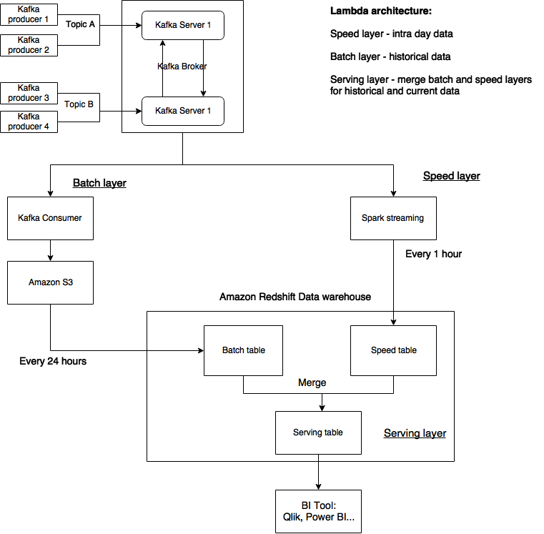
You can observe the three main layers in the following example of the architecture:

Data ingestion implementation

Streaming data is ingested using Apache Kafka.

Kafka provides immutable, persisted and replicated short term storage of data.

The data is then forwarded to various consumers who subscribe to relevant topics.

Speed layer implementation

Streaming data in consumed every couple of minutes using Structured Spark Streaming.

The data from the start of the day until current time is aggregated every hour and the results of aggregation are exported (overwrite) into the Speed view table on Amazon Redshift (marked as Speed table in drawing).

Batch layer implementation

Streaming data is incrementally consumed every couple of hours using a Kafka Consumer.

The data is then uploaded to S3 object storage which serves as cheap long term storage.

Directly from S3 the data is also imported into Redshift “raw_batch” table.

This “raw batch” table is then aggregated to produce the Batch view which has the same definition as Speed view.

Compared to the Speed view, the Batch view is produced once a day based on all historical data.

Serving layer implementation

Batch view contains the aggregations of all historical data except the data for today and the Speed view contains only the aggregation of todays data.

Serving layer combines the aggregations found in Batch and Speed view to enable the consumption of most recent intraday data as well as all historical data.

Since both views share the same definition they can be easily merged using SQL commands on Amazon Redshift.

You can find the code from this blog post in this github repository.